Vehicle Detection Project
The notes for this project are best viewed on line at the github repo. It is easier to follow the links to the source code referenced in this documentation. This readme is my completion of the Udacity project template provided at this repo.
The project code is developed using the spyder IDE and is made up of the following files.
- detect_vehicles.py - The main vehicle detection module. The functions used to process various videos while varying some parameters.
- gen_output.py - Script used during the development and debug phase for visualization and used to generate the images used for the documentation.
- utils.py and config.py - Utility procedures and setup information.
- lesson_functions.py - The module that contains the procedures provided in the Udacity Self-Driving Car Engineer Nanodegree lecture notes.
The following steps are done to complete this project.
- A Linear SVC classifier is trained on a set of images labeled as cars and not-cars.
- A feature vector made up of the following features is used for training.
- A Histogram of Oriented Gradients (HOG),
- A color transform with binned colors
- A histograms of color
- The feature vector is normalized and randomized before training and testing.
- Vehicles are identify in an image by using a sliding-window technique to segment the image into blocks that are fed into the trained classifier.
- The above process is applied to the images in a video stream to identify the cars.
- A heat map identifies the locations of cars by summing all the blocks within an image that is identified as a car.
- The heat map is also calculated from the last 20 fames of the image in order to reject outliers and follow detected vehicles.
- Bounding boxes are drawn around detected vehicles.
- The above procedure was run on project_video.mp4
Histogram of Oriented Gradients (HOG)
The
get_hog_features
function was called in order to generate the HOG images for an image
in the vehicle and non-vehicle class.
The
select_example_images
function was use to select the middle images from the small training data set
in order to get a feel for what the skimage.feature.hog() output looks like.
The
gen_hog
function calls the
get_hog_features
function to generate the images below.
The following example images are converted to gray scale and the HOG features are detected
with the following parameters orientations=9, pixels_per_cell=(8, 8) and cells_per_block=(2, 2).
| Car | Car HOG | Not Car | Not Car HOG |
|---|---|---|---|
 |
 |
 |
 |
The
train_svm
function used the hog parameters noted above to train and test a LinearSVC.
The SVC was trained by reading in the vehicle and non-vehicle images
and extracting the features, scaling them and then fitting them to the
classifier.
The test data was run through the classifier in order to see the accuracy
of the predictions based on the hog parameters selected.
The predictions for the HOG parameters noted above was determined to be
adequate when used with the large training data set.
Along with the HOG features, a color histogram and spatial binning of the image were combined and used as features.
Sliding Window Search
A sliding window was used on the test images in order to detect the cars.
The sub-sampling, of the full image HOG features, was used on the test
images in oder to speed up the image detection.
The
find_cars
function shows how the sub-sampling was used to determine the bounding box for the cars
using the parameter that were determined in the previous section.
The cells_per_step parameter was used to determine the overlap between the
sliding windows.
The get_cars function calls the find_cars functions twice with a scale of 1 and 1.5 in order to detect cars near and far. Other values of scale can be used but were not necessary in order to detect the cars correctly for the project video provided. The get_cars function also averaged the cars detected over a number of frames and will be explained in the next section. To improve the reliability of the classifier a number of feature combinations were tested with the test images provided. The configuration file shows some of the features that were tested out.
After the experimentation noted above the following features were selected for the feature vector:
- a YCrCb 3-channel HOG features at two scales,
- a 32x32 spatially binned color features and
- a 32 bin histograms of 255 color features.
Heat map thresholding was used to reduce the multiple detects caused by overlapping sliding windows and also by overlapping windows due to multiple scales. The example images below show the multiple detects (blue box) and the heat map threshold reduced to a single detect (white box).
| test1.jpg | test3.jpg | test4.jpg | test4.jpg |
|---|---|---|---|
 |
 |
 |
 |
Video Implementation
Here is a local link to the result video and a youtube video link.
In order to create the video shown at the link above, you first train and save the classifier via:
./detect_vehicles.py -d big -c 15 train
then you use the trained classifier on the project video by using the command shown below.
./detect_vehicles.py -d big -c 15 video -i 7 -t 16
In the
get_cars
function the positions of the detections in each frame of the video
are stored for 20 consecutive frames in a FIFO.
A heat map is then created for the 20 frame history and a threshold of 16 is used
to identify a vehicle's position and filter out the transient false positives.
The scipy.ndimage.measurements.label() is used in the
heat_map
function to identify individual cars in the heat map.
A bounding box is drawn around the area where a car is detected.
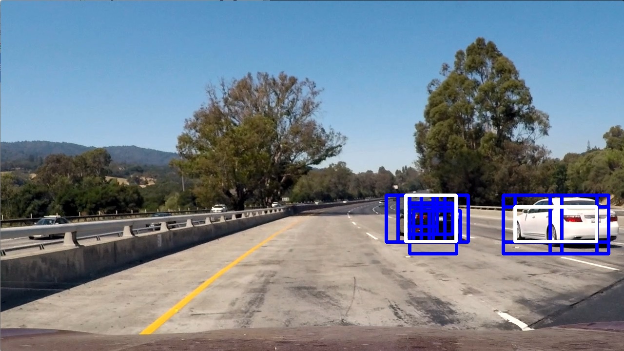
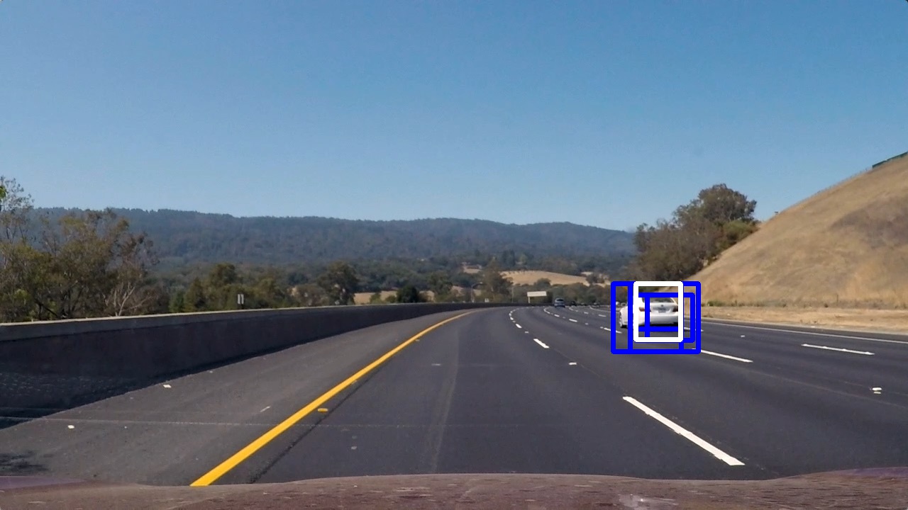
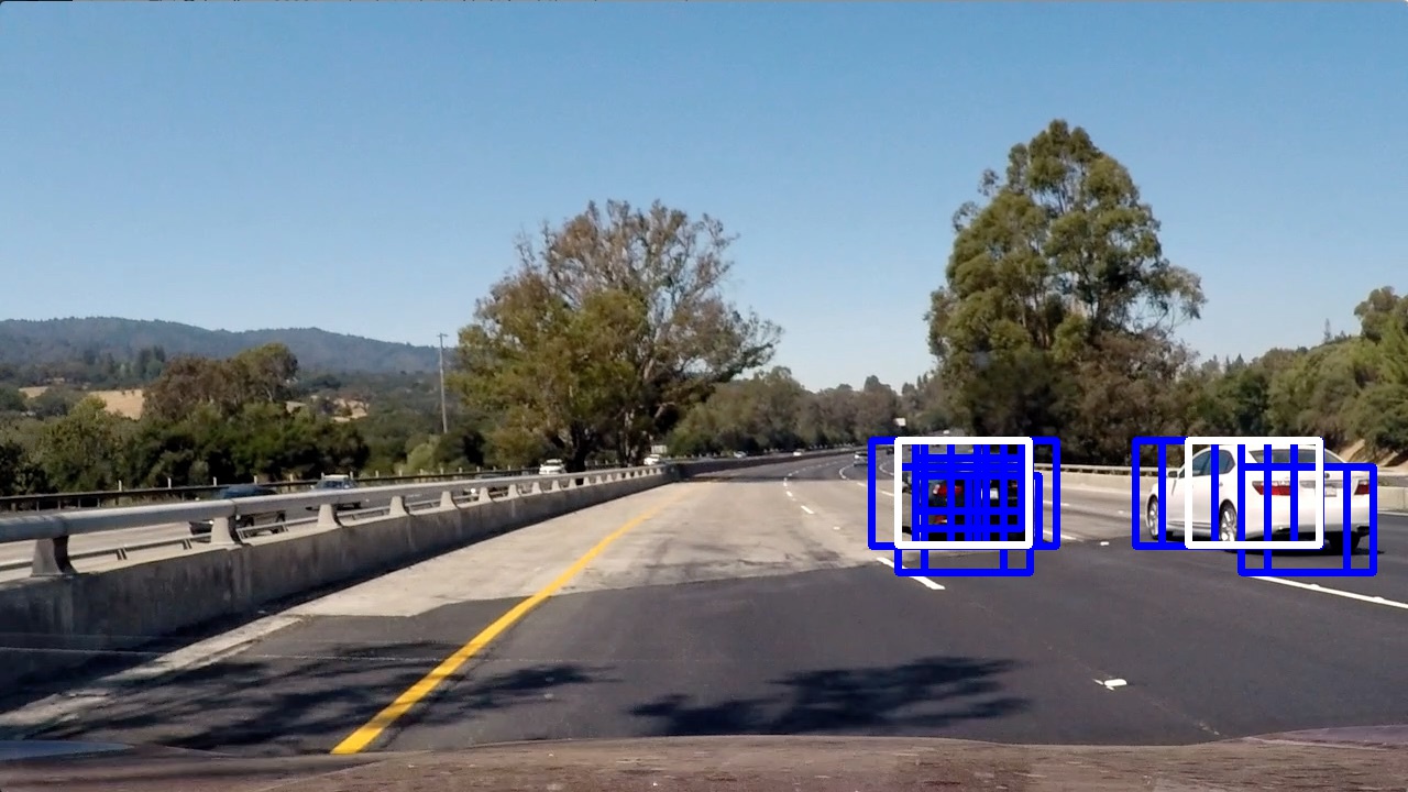
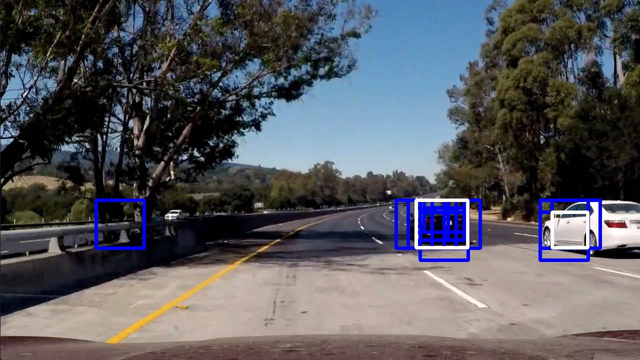
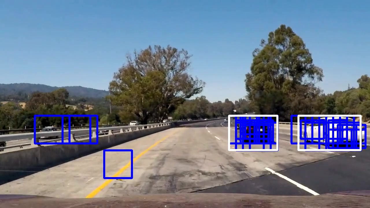
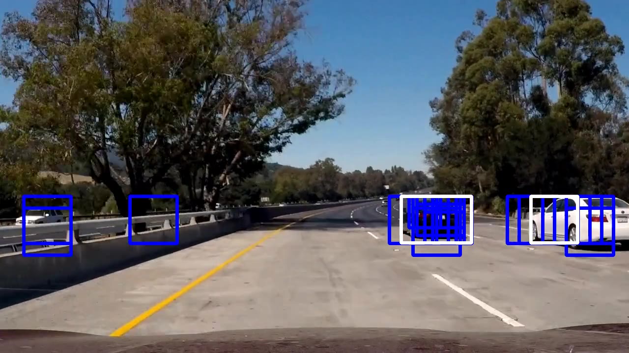
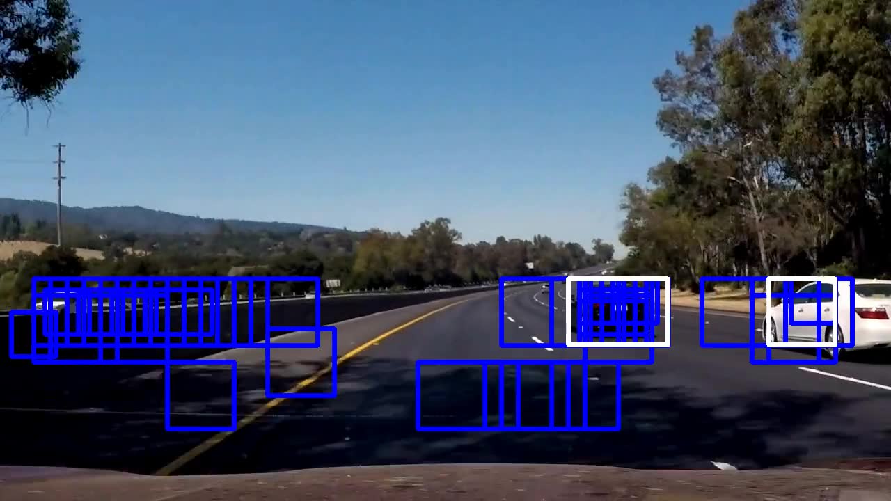
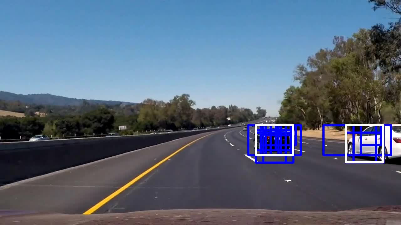
The images below show the operation of the algorithm.
The blue boxes shows the detections over 20 frames and the white boxes
are the ones actually drawn on the video because they surpass the heat threshold.
| image004.jpg | image005.jpg | image005.jpg | image007.jpg |
|---|---|---|---|
 |
 |
 |
 |
Discussion
A major issue in this project, is that in order to adequately test all the possible parameters, that one can vary before and after training the classifier, takes quite a bit of compute time per iteration.
Even with all that effort it is easy to see that this pipeline can fail if:
- there were extreme shadows
- the lighting condition varied from day to night or
- trees or shrubs are present on the side of the road.
A straight forward way to improve this project is to test it with videos the have the properties noted above and tune the parameters for the highly changing environment.